Managed Server(bi_server1) start with ADMIN state in OBIEE

Dear All,

Recently one fine day we found that our BI application suddenly stopped working, we didn’t find the root cause . But While using the universe best solution ‘RESTART’, We found that Managed server starting in ADMIN state instead of RUNNING. Google Guru has given us some idea that it is because of some db connection issue and server is failing to start some component.

Problem Statement: Managed Server(bi_server1) start with ADMIN state

Resolution: Checked the logs for weblogic server and get to know that some of the Data sources are throwing TNS error while starting the component.

For Example:

<<WLS Kernel>> <> <b4cb6966a5479011:-6e64bb28:150530bc594:-8000-000000000001124a> <1444642299486> <BEA-001129> <Received exception while creating connection for pool “EPMSystemRegistry-rac1”: Listener refused the connection with the following error: ORA-12514, TNS:listener does not currently know of service requested in connect descriptor.

History:

Data-base was set up on 2 server isntances(RAC) and Issue was that one of the database RAC(instance) gone down and due to this server was not able to connect to DB and the component which were using that RAC were throwing

Resolution:

Changed the TNS details in component and configured the running and active DB details. Changed the parameter in Weblogic Console URL at location: Home > Summary of Services > Summary of JDBC Data sources

Restarted the all the component and good to see that Bi_server1 was up and running.

However Now encountered a new issue that EM URL(http://localhost:1000/em) was not opening.

Get to know that EM.ear file which is deployed in Console are corrupted and due to this EM URL was not working. Re-deployed the EM.ear file in deployment section and good to see that EM URL was up and running.

Eventually our problem didn’t end here, while trying to login in OBIEE analytic we found that no user is able to login into OBIEE even Weblogic also.

Checked all the related log files like biserver, presentation_server etc and get  error like authentication failed, wrong user name password error etc.

From my past experience I realized that:

• might be MDS and BIPLATFORM password expire/locked  but it was not true. Both the schema were in open state.
• might be BISystemUser is corrupted, basically this user is responsible for bi_component internal communication. I changed the password for this user in Console and updated the same in EM security credentials section however no luck still.

Resolution:

Created a new user in Console as BISystemUser1 (can give any name). Then replaced the existing BISystemUser details in EM( oracle.bi.system credential map, select system.user and click Edit) with BISystemUser1 details.

Started all the components again and Finally we were able to login in OBIEE analytic.

Thanks,

Deependra (Deep’sa )

Be Happy….Be Healthy

 

 

Rapidly Changing Monster Dimension – Mini Dimension In Data Warehousing

Traditional Data Warehouse often experience a scenario where we need implementation of Mini Dimension. We found a textbook definition of Mini Dimension in Kimball Group here. We often consider this as Slowly Changing Dimension Type 4, a good reference of different SCD types can be found here in Kimball group as well.

We would like to discuss about a practical demand scenario for Mini Dimension implementation and also we would discuss an implementation plan for Mini Dimension in a typical BI Project. As we know “Necessity is the mother of Invention” , we would first understand the problem statement in a typical DWH Reporting Environment without Mini Dimension and then we would look into the approaches to resolve that problem statement using Mini Dimension.

Scenario:

If we assume a typical Order Entity which consist of Order Number, Order Type, Order Status, Order Category etc. and if we create an Order Dimension consist of all of these attributes then any fact consist of Order Dimension’s foreign key can relate to these attributes and they can be used for slicing the reporting measures.

If we consider any need of Aggregate creation which is in rolled up level of Order Transaction(anything which has higher granularity than Order Transaction e.g. Weekly Count of Orders Created), and if we need slicing that measure as well, then it would be a likely situation where we can use Mini Dimension.

Example:

Requirement on Day 1 – Reporting on # of Orders per week per Order Type

We design Aggregate Table with columns – # of Orders, Week Id, Order Type

Then the Requirement got amended on Day 2 –  Reporting on # of Orders per week per Order Type and Order Status.

To cope up with this change we need to change Aggregate Table structure to add a new slicing attribute Order Status.

And Business Customers can ask for these type of Slicing Attributes more frequently, so this is obvious that we should not put these slicing attributes in Aggregate table, rather we should create another dimension with only slicing attributes and store foreign key into its Original Dimension and Aggregate Table. This will give more flexibility to Data Model we can cope up with frequent ask for different slicing Attributes in the report.

Candidates for Mini Dimension Attributes:

As per Kimball Group – “Slowly changing dimension type 4 is used when a group of attributes in a dimension rapidly changes and is split off to a mini–dimension. This situation is sometimes called a rapidly changing monster dimension. Frequently used attributes in multimillion-row dimension tables are mini-dimension design candidates, even if they don’t frequently change. The type 4 mini-dimension requires its own unique primary key; the primary keys of both the base dimension and mini-dimension are captured in the associated fact tables.”

Practically we can use another technique to identify whether an attribute can be considered in one of those few “elite” members in Mini Dimension. If we check cardinality of any column in table, whatever the columns with very low cardinality are present in that table, will be considered for Mini Dimension. So if we draw histogram of all the columns in a table, the lower bars are the suitable candidate for Mini Dimension Attributes.

Technique for Implementation:

Step 1 >> Identify Mini Dimension Candidates

Step 2 >> Populate Mini Dimension

==================================================

merge  into <Mini Dimension Table Name> tgt
using
(
select
distinct

<Set of Identified Columns>

from wc_order_ds a — This is Incremental Dimensional Data Set
) src
on
(

–Match Identified Columns in existing Mini Dimension table for capturing any new combination. Example as follows

NVL(TGT.order_status,’X’) = NVL(SRC.order_status,’X’) AND
NVL(TGT.fulflmnt_status,’X’) = NVL(SRC.fulflmnt_status,’X’) AND
NVL(TGT.order_type,’X’) = NVL(SRC.order_type,’X’)

)
when not matched then
insert
(
row_wid, — Mini Dimension Surrogate Key

<Mini Dimension Columns>
)
values
(
<Sequence Name>.nextval, — Sequence Number to populate Surrogate Key
src.<Mini Dimension Columns>

);
commit;

===================================================

Step 3 >>  Add MINI_WID (Mini Dimension’s Primary Key) Into Dimension

========================================================
MERGE /*+ PARALLEL (TGT,4) */ INTO WC_ORDER_D TGT
USING
(

SELECT /*+ PARALLEL(TGT,4) */
TGT.<Target Column List>
SRC.ROW_WID AS MINI_WID
FROM WC_ORDER_DS TGT, — Order Dimension Incremental Table
WC_ORIG_ORDER_MD SRC — Mini Dimension Table
where

<Matching the Mini Dimension Attributes for getting MINI_WID>
NVL(TGT.order_status,’X’) = NVL(SRC.order_status,’X’) AND
NVL(TGT.fulflmnt_status,’X’) = NVL(SRC.fulflmnt_status,’X’) AND
NVL(TGT.channel,’X’) = NVL(SRC.channel,’X’)
) STG
ON
(
<Matching Criteria for Target and Incremental Set>

)
WHEN NOT MATCHED
THEN
INSERT
(

<Target Columns>

MINI_WID
)
VALUES
(
<Target Columns>

STG.MINI_WID
);

=======================================================

Step 4 >> Add Mini WID into Fact table as well. This step can be done appending one another column (MINI_WID) from Dimension while Populating Fact’s Foreign Key (Dimension’s ROW_WID ). This Step is optional, we can avoid this step if we want to, because in any case we can add dimension table in the query while populating aggregate table, and select MINI_WID from Dimension, but if it present in Fact then we can directly select it from Fact while Aggregating. This decision is purely based on Design Scenario and we need to choose the optimal design approach.

Step 5 >> Add MINI_WID into Aggregate table.

Step 6 >> 

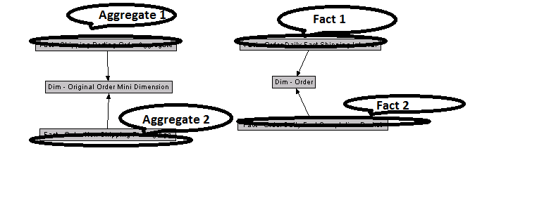
In BI Data Model (In RPD as we use OBIEE) we need to join Aggrgate table with Mini Dimension and Fact table needs to be joined with Dimension Table, so that summary reports can be directly fetched from Mini Dimension and Aggregate tables, and only detail reports will be generated from Fact and Dimension Tables. This will add advantage on Performance Perspective as well..

Example:

Mini Dimension with Aggregates in RPD Physical Layer

Step 7 >> We can create a dimension Hierarchy for Mini Dimension Attributes as Order Attributes which would be the parent level of Order Detail.

Step 8 >> Set Content Level for Order Dimension in Aggregate Tables as Order Attributes and in Fact Tables as Order Detail.

Step 9 >> Build Summary and Detail Report as required

Step 10 >> Enjoy the speed and power of Mini Dimension in your report

Hope the above post would help to identify the opportunities of implementing Mini Dimension in real BI Project Scenario.

Please feel free to comment your thinking and any other approaches for these scenarios..

Happy reading!!..

Cheers!!!

Regards,

Sourish

Dimension Based Aggregation Rule in OBIEE – Part 2 – Ordering is important

We have already discussed about how to achieve Dimension based Aggregation Rule in OBIEE here. And we have also had a glimpse on ordering of selected dimension. We will discuss about ordering of dimension based rule and how that changes the physical sql in OBIEE and which in turn changes the outcome of analysis.

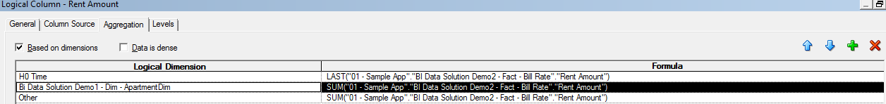
Let us start where we had ended our last discussion, we had created 3 dimension based rules as following order:

Dimension Based Aggregation Ordering

And the above setting yields the physical sql which is selecting the last rent for every house and then sum it up.

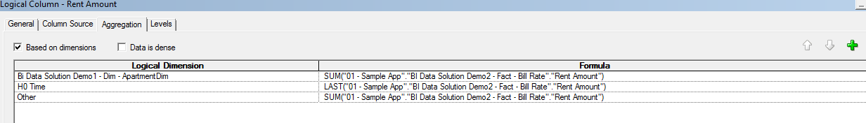
Let us re-order the dimension rules as follows:

Here we have set the summation of house as the first rule and then selection of last on time slice.

And this ordering yields the below physical sql:

========================================

WITH
SAWITH0 AS (select T42404.Per_Name_Month as c2,
T285805.HOME_ID as c4,
T285805.RESIDENT_NAME as c5,
T285805.APARTMENT_ID as c7,
T42404.Per_Name_Qtr as c9,
sum(T285817.RENT_AMOUNT) as c10,
T42404.Calendar_Date as c13
from
BISAMPLE.WC_APARTMENT_D T285805 /* Bi Data Solution Demo1 – Dim – Apartment */ ,
BISAMPLE.SAMP_TIME_DAY_D T42404 /* D01 Time Day Grain */ ,
BISAMPLE.BILL_RATE_FACT T285817 /* BI Data Solution Demo2 – Fact – Bill Rate */
where ( T42404.Day_Key = T285817.DAY_WID and T285805.ROW_WID = T285817.APARTMENT_WID )
group by T42404.Calendar_Date, T42404.Per_Name_Month, T42404.Per_Name_Qtr, T285805.APARTMENT_ID, T285805.HOME_ID, T285805.RESIDENT_NAME),
SAWITH1 AS (select D1.c2 as c2,
D1.c4 as c4,
D1.c5 as c5,
D1.c7 as c7,
D1.c9 as c9,
sum(D1.c10) over (partition by D1.c13) as c10,
sum(D1.c10) over (partition by D1.c13, D1.c7, D1.c4, D1.c5) as c11,
sum(D1.c10) over (partition by D1.c13, D1.c7) as c12,
D1.c13 as c13
from
SAWITH0 D1),
SAWITH2 AS (select distinct LAST_VALUE(D1.c10 IGNORE NULLS) OVER (PARTITION BY D1.c2, D1.c9 ORDER BY D1.c2 NULLS FIRST, D1.c9 NULLS FIRST, D1.c13 NULLS FIRST ROWS BETWEEN UNBOUNDED PRECEDING AND UNBOUNDED FOLLOWING) as c1,
D1.c2 as c2,
LAST_VALUE(D1.c11 IGNORE NULLS) OVER (PARTITION BY D1.c7, D1.c4, D1.c5, D1.c2, D1.c9 ORDER BY D1.c7 NULLS FIRST, D1.c4 NULLS FIRST, D1.c5 NULLS FIRST, D1.c2 NULLS FIRST, D1.c9 NULLS FIRST, D1.c13 NULLS FIRST ROWS BETWEEN UNBOUNDED PRECEDING AND UNBOUNDED FOLLOWING) as c3,
D1.c4 as c4,
D1.c5 as c5,
LAST_VALUE(D1.c12 IGNORE NULLS) OVER (PARTITION BY D1.c7, D1.c2, D1.c9 ORDER BY D1.c7 NULLS FIRST, D1.c2 NULLS FIRST, D1.c9 NULLS FIRST, D1.c13 NULLS FIRST ROWS BETWEEN UNBOUNDED PRECEDING AND UNBOUNDED FOLLOWING) as c6,
D1.c7 as c7,
LAST_VALUE(D1.c10 IGNORE NULLS) OVER (PARTITION BY D1.c9 ORDER BY D1.c9 NULLS FIRST, D1.c13 NULLS FIRST ROWS BETWEEN UNBOUNDED PRECEDING AND UNBOUNDED FOLLOWING) as c8,
D1.c9 as c9
from
SAWITH1 D1),
SAWITH3 AS (select sum(T285817.RENT_AMOUNT) as c3,
T42404.Calendar_Date as c4
from
BISAMPLE.SAMP_TIME_DAY_D T42404 /* D01 Time Day Grain */ ,
BISAMPLE.BILL_RATE_FACT T285817 /* BI Data Solution Demo2 – Fact – Bill Rate */
where ( T42404.Day_Key = T285817.DAY_WID )
group by T42404.Calendar_Date),
SAWITH4 AS (select LAST_VALUE(D1.c3 IGNORE NULLS) OVER ( ORDER BY D1.c4 NULLS FIRST ROWS BETWEEN UNBOUNDED PRECEDING AND UNBOUNDED FOLLOWING) as c2
from
SAWITH3 D1),
SAWITH5 AS (select max(D1.c2) as c1
from
SAWITH4 D1),
SAWITH6 AS (select D1.c7 as c2,
D1.c4 as c3,
D1.c5 as c4,
D1.c2 as c5,
D1.c9 as c6,
D1.c3 as c7,
max(D1.c6) as c8,
max(D1.c8) as c9,
max(D1.c1) as c10,
D2.c1 as c11
from
SAWITH2 D1,
SAWITH5 D2
group by D1.c2, D1.c3, D1.c4, D1.c5, D1.c7, D1.c9, D2.c1),
SAWITH7 AS (select D1.c1 as c1,
D1.c2 as c2,
D1.c3 as c3,
D1.c4 as c4,
D1.c5 as c5,
D1.c6 as c6,
D1.c7 as c7,
D1.c8 as c8,
D1.c9 as c9,
D1.c10 as c10,
D1.c11 as c11
from
(select 0 as c1,
D1.c2 as c2,
D1.c3 as c3,
D1.c4 as c4,
D1.c5 as c5,
D1.c6 as c6,
D1.c7 as c7,
max(D1.c8) over (partition by D1.c5, D1.c6, D1.c2) as c8,
max(D1.c9) over (partition by D1.c6) as c9,
max(D1.c10) over (partition by D1.c5, D1.c6) as c10,
D1.c11 as c11,
ROW_NUMBER() OVER (PARTITION BY D1.c2, D1.c3, D1.c4, D1.c5, D1.c6 ORDER BY D1.c2 ASC, D1.c3 ASC, D1.c4 ASC, D1.c5 ASC, D1.c6 ASC) as c12
from
SAWITH6 D1
) D1
where ( D1.c12 = 1 ) )
select D1.c1 as c1, D1.c2 as c2, D1.c3 as c3, D1.c4 as c4, D1.c5 as c5, D1.c6 as c6, D1.c7 as c7, D1.c8 as c8, D1.c9 as c9, D1.c10 as c10, D1.c11 as c11 from ( select D1.c1 as c1,
D1.c2 as c2,
D1.c3 as c3,
D1.c4 as c4,
D1.c5 as c5,
D1.c6 as c6,
D1.c7 as c7,
D1.c8 as c8,
D1.c9 as c9,
D1.c10 as c10,
D1.c11 as c11
from
SAWITH7 D1
order by c1, c6, c5, c2, c3, c4 ) D1 where rownum <= 5000001

====================================

As per the above physical sql – we are selecting the sum() with group by on the other attributes in the innermost query segment and then in subsequent steps we are selecting the last() value of that measure.

It is basically selecting as follows:

Step 1:

a) All rent for Q1 (10,20,30,40)

b) All rent for Q2 (10,20,30)

c) All rent for Q3 (10,20,30)

Step 2:

Selecting the last summation from Step 1 (i.e. c) All rent for Q3 (10,20,30))

So the resulting analysis is as following:

Last Time’s Rent

If we look at the Grand Total – it is only 3140 which is the total of Q3 only (House number 40 is excluded as it was on last Q1).

By discussing the above technique we have now understood how we can use this in our favor to produce different insight of data, and we love data because it gives us more valuable information than the entity/incident itself.

Former CEO of HP, Carly Florina once said – “The goal is to turn data into information, and information into insight.” , and this is exactly we want to do using BI and Analytics.

Hope you have enjoyed reading and please share your comments and feedback..

Happy Reading..Bye!!!

Thanks and regards,

Sourish

Dimension Based Aggregation Rule in OBIEE – Part 1 – How to

Aggregation rule is a key feature in OBIEE which enables technique of rolling up  data in different level. We can discuss about OBIEE Aggregation Rule for Measure values in a separate post which will have a broader scope. Today I would like to share my experience with Dimension Based Aggregation Rule in OBIEE.

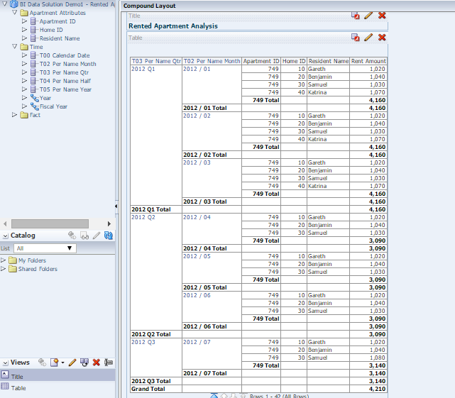
Let us consider a scenario of Rented Apartments where the analysis should show Time Attributes (Quarter.month etc), Apartment Attributes (Apartment Number, House Number, Tenant Name etc) along with the Rent amount by Time Slice and Apartments with a specific aggregation rule – Roll up All House’s Latest Rent which is depicted below :

Summation of All House’s Latest Rent

As you can see above in Q1 there were 4 houses (10,20,30 and 40) and total rent was 4160, in Q2 there were only 3 houses (house number 40 was empty probably!!) and total rent was 3090 . In Q3 landlord increased the rent for House number 30 and Samuel had to give 1,080 bucks and total rent amount for Q3 became 3140.

Now if we calculate All House’s Latest Rent then it would be –

House 10 – 1020 bucks in Q3

House 20 – 1040 bucks in Q3

House 30 – 1080 bucks (Poor Samuel!!) in Q3

House 40 – 1070 bucks (Katrina already shifted her house) in Q1

===================================================

Total – 4210 bucks

===================================================

Data model for this analysis is very simple, Apartment Dimension, Time Dimension (Day. Month, Quarter grain) and Rent Fact as below:

Rented Apartment Data Model

As we can see there are different aggregation rule required for different dimensions – select latest rent for time basis i.e. use of last() and select total rent for house basis i.e. use of sum(). Only one aggregation rule is not sufficient here and it will produce wrong result.

So we need to use dimension based aggregation rule as shown below:

Dimension Based Aggregation

After ticking the above marked check box (Based on dimensions) we need to set different aggregation rule for different dimensions as below:

Dimension Based Aggregation Ordering

As we can see that we are using different dimensions here so creation of dimension hierarchy (logical dimension) is a prerequisite. And also please note OBIEE Best Practice always encourage to create Logical Dimension for each and every Dimension Table and fill up the content level with proper dimension level information..these can be discussed in detail later.

After deploying this RPD, we have created one sample analysis and ensured that the aggregation rule (in result tab) of the metric is set to Default. And the Analysis Result was shown at the first picture. Let us now check the physical SQL for this analysis-

===================

WITH
OBICOMMON0 AS (select distinct T285805.HOME_ID as c2,
T285805.RESIDENT_NAME as c3,
T42404.Per_Name_Qtr as c5,
T285805.APARTMENT_ID as c6,
LAST_VALUE(T285817.RENT_AMOUNT IGNORE NULLS) OVER (PARTITION BY T285805.ROW_WID, T42404.Per_Name_Qtr ORDER BY T285805.ROW_WID NULLS FIRST, T42404.Per_Name_Qtr NULLS FIRST, T42404.Calendar_Date NULLS FIRST ROWS BETWEEN UNBOUNDED PRECEDING AND UNBOUNDED FOLLOWING) as c7,
T285805.ROW_WID as c8,
LAST_VALUE(T285817.RENT_AMOUNT IGNORE NULLS) OVER (PARTITION BY T285805.ROW_WID ORDER BY T285805.ROW_WID NULLS FIRST, T42404.Calendar_Date NULLS FIRST ROWS BETWEEN UNBOUNDED PRECEDING AND UNBOUNDED FOLLOWING) as c9
from
BISAMPLE.WC_APARTMENT_D T285805 /* Bi Data Solution Demo1 – Dim – Apartment */ ,
BISAMPLE.SAMP_TIME_DAY_D T42404 /* D01 Time Day Grain */ ,
BISAMPLE.BILL_RATE_FACT T285817 /* BI Data Solution Demo2 – Fact – Bill Rate */
where ( T42404.Day_Key = T285817.DAY_WID and T285805.ROW_WID = T285817.APARTMENT_WID ) ),
SAWITH0 AS (select D1.c2 as c2,
D1.c3 as c3,
D1.c5 as c5,
D1.c6 as c6,
D1.c7 as c7,
D1.c8 as c8,
ROW_NUMBER() OVER (PARTITION BY D1.c2, D1.c3, D1.c5, D1.c6, D1.c8 ORDER BY D1.c2 DESC, D1.c3 DESC, D1.c5 DESC, D1.c6 DESC, D1.c8 DESC) as c9,
ROW_NUMBER() OVER (PARTITION BY D1.c5, D1.c6, D1.c8 ORDER BY D1.c5 DESC, D1.c6 DESC, D1.c8 DESC) as c10
from
OBICOMMON0 D1),
SAWITH1 AS (select sum(case D1.c9 when 1 then D1.c7 else NULL end ) as c1,
D1.c2 as c2,
D1.c3 as c3,
sum(case D1.c10 when 1 then D1.c7 else NULL end ) as c4,
D1.c5 as c5,
D1.c6 as c6
from
SAWITH0 D1
group by D1.c2, D1.c3, D1.c5, D1.c6),
SAWITH2 AS (select D1.c1 as c1,
D1.c2 as c2,
D1.c3 as c3,
sum(D1.c4) over (partition by D1.c5, D1.c6) as c4,
D1.c5 as c5,
D1.c6 as c6
from
SAWITH1 D1),
SAWITH3 AS (select D1.c9 as c2,
D1.c8 as c3,
ROW_NUMBER() OVER (PARTITION BY D1.c8 ORDER BY D1.c8 DESC) as c4
from
OBICOMMON0 D1),
SAWITH4 AS (select sum(case D1.c4 when 1 then D1.c2 else NULL end ) as c1
from
SAWITH3 D1),
SAWITH5 AS (select D1.c6 as c2,
D1.c2 as c3,
D1.c3 as c4,
D1.c5 as c5,
D1.c1 as c6,
max(D1.c4) as c7,
max(D2.c1) as c8
from
SAWITH2 D1,
SAWITH4 D2
group by D1.c1, D1.c2, D1.c3, D1.c5, D1.c6),
SAWITH6 AS (select D1.c1 as c1,
D1.c2 as c2,
D1.c3 as c3,
D1.c4 as c4,
D1.c5 as c5,
D1.c6 as c6,
D1.c7 as c7,
D1.c8 as c8
from
(select 0 as c1,
D1.c2 as c2,
D1.c3 as c3,
D1.c4 as c4,
D1.c5 as c5,
D1.c6 as c6,
max(D1.c7) over (partition by D1.c5, D1.c2) as c7,
max(D1.c8) over () as c8,
ROW_NUMBER() OVER (PARTITION BY D1.c2, D1.c3, D1.c4, D1.c5 ORDER BY D1.c2 ASC, D1.c3 ASC, D1.c4 ASC, D1.c5 ASC) as c9
from
SAWITH5 D1
) D1
where ( D1.c9 = 1 ) )
select D1.c1 as c1, D1.c2 as c2, D1.c3 as c3, D1.c4 as c4, D1.c5 as c5, D1.c6 as c6, D1.c7 as c7, D1.c8 as c8 from ( select D1.c1 as c1,
D1.c2 as c2,
D1.c3 as c3,
D1.c4 as c4,
D1.c5 as c5,
D1.c6 as c6,
D1.c7 as c7,
D1.c8 as c8
from
SAWITH6 D1
order by c1, c5, c2, c3, c4 ) D1 where rownum <= 5000001

===========================

Here please note that the innermost query is executing last() function , which we have set as the first precedence while setting dimension based aggregation rule and then in the outer part it is executing sum() function.

By this way the OBIEE server first selecting the latest rent for every house (10,20,30 and including 40) and then rolling up the latest rents as total rent.

Here we have got a glimpse of the fact that – Ordering is important in Dimension Based Aggregation rule, we will discuss that in our next post.

Till then Happy Renting !! Oops…Happy Reading !!

Regards,

Sourish

Date format set for LOCAL TIME ZONE in OBIEE

Hello,

Its quite interesting that I got a chance to work with different time zone customers and everywhere the  first feedback from Tester/user I get on report is Please.. Please…. Change the Date format.

For Example User from UK time zone will ask, currently date in prompt is showing MM/DD/YYYY as per default configuration whereas we want it in DD/MM/YYYY format. And changed the same for ad-hoc reporting also(for all the date column in webcat).

There are couple of ways to achieve this:

1. First Method: At column level: This is quite lazy method, here we have to go to column properties of individual column at  reporting side and need to change the data format as shown below but the good thing about this method is we can give any format to date column at run time.

Column Data Format

2. Second Method: Asked the end-user to change the preferences in My Account, change the Time Zone for UK.

Above 2 methods are not well suited for large set of customer and columns.

So the finest method to set the LOCAL Date fromat across the webcat for all the customer from the same zone is below:

1. Set the USERLOCALE system session variable in RPD. And this will change the date format to UK time zone(DD/MM/YYYY) for all date column across webcat. Below the one step method.

USER LOCALE Initialization Block

Set the appropriate zone value in Initialization block above example is for ‘gb’ – Great Britain.

Be Happy….Be Healthy…..

Thanks, Deepsa

ORA_HASH for ETL improved performance.

Amateur blogger, read carefully. 

Problem Scenario:
1. There are cases when we pull the data from OLTP source through DB link or in huge quantity.
Its happens many times that connection get breaks and network congestion increase and takes huge time before committing the complete transaction and because of this some time we loose the uncommitted data.
2. Or some time because the transaction frequency is high and due to this your select statement is not able to read from redo log as fast as expected.

Solution approach:

One of the solution approach for above said problem scenario is divide/partition the data in small chunks through some function and then select and insert the data in the target table in small-small chunks

Solution(Tested scenario) based on ORA_HASH :

ORA_HASH is a function that computes a hash value for a given expression. This function is useful for operations such as analyzing a subset of data, generating a random sample and selection of data-set. It always return a number value and use HASH_PARTITIONS algorithm.

Syntax: ORA_HASH(Expression, max_bucket, seed_value);

For more information on ORA_HASH kindly see: http://docs.oracle.com/cd/B12037_01/server.101/b10759/functions097.htm

We can use basic functionality of ORA_HASH function with FOR LOOP and get the hash value number for a row and then select, insert and commit in bunches.

For Example:

BEGIN

for i in 0 .. 7
loop
insert into Table ABC
(
column A,
column B
)
select
column A.p,
column B.q
from table A, table B
where 1=1 and A.row_id = B.row_id and
ORA_HASH (A.row_wid,7,0)=i;

end loop;

commit;

END;
/

Result : In above example suppose Select statement on Table A and Table B is returning 1 Mn record which is a big count and selecting, transferring and Inserting 1 Mn records through DB link is time-consuming, heavy on network.
What I have done here is divided the Complete set of data(1Mn) in almost 8 equal sets(around 120K) and based on FOR LOOP inserting in the target table in small-small chunks.

Kindly do comment.

Object Oriented Programming approach in OBIEE – LTS Overriding – Part 2

We had discussed in my previous post here about one real life project scenario where we need to build a report with mixed granularity (e.g. report will have Order Detail and Product detail), but the same time your data model should be consistent and perform (report data returning time) well enough to support simplest form of report (e.g. only Order Details).

We have already built couple of LTS in the same Logical Table (lets assume Logical Table for Dimension C – Order). Prior to look into the fact how we override the LTS , let us briefly recollect our concept of Overriding in OOP. Though Object Oriented Programming concept is not in the scope of this post, but one good example I’ve found in internet here , you may find it useful to just brush up the concept once again.

To solve the aforementioned business problem, let us consider that we would need two LTS in the same Logical Table for Dimension C. One LTS with standalone Dimension C table and another with 3 tables (Dimension C, Fact B and Dimension D). Those two LTS are depicted below once again for reference

Simplest form of LTS

LTS for accommodating other tables

Now we need to set Dimension C (Order Dimension) related logical columns to both of these two LTS , so that if we pull only Order attribute related column in report then OBIEE would only select Dim – Order Standalone LTS (simpler LTS). When we would pull any Product related attributes along with Order attribute OBIEE would access the Dim – Order Line Item LTS (complex LTS). And we can ensure this with configuring the priority, so that the simpler LTS gets higher priority 0 (Super Class in OOP) and complex LTS gets lower priority  3 (sub class in OOP).

Logical Column Source from different LTS

Now let us think the above scenario in Object Oriented Programming world.

In object Oriented Programming world we can think these two LTS as two class :

Dim – Order Standalone –> superclass

{

Method of the super class  yields Joining Tables –> Only Dimension C (Order Dimension) in this case

);

Dim – Order Line Item  –> Subclass

This class extends its superclass Dim – Order Standalone

{

Method of the super class  yields Joining Tables –> Dimension C , Fact B and  Dimension D in this case

);

When we pull Product related attribute then we instantiate an Object of Subclass Dim – Order Line Item but in case of simpler reports we instantiate an object of Superclass Dim – Order Standalone. Thus we can achieve the dynamic selection of joining tables depending on the reporting attributes , implementing LTS Overriding as in Object Oriented Programming .

The above mentioned technique can be used to resolve these kind of business problem where we need to decide dynamically which physical tables we need to join to get the consistent data in more efficient way.

Hope you have enjoyed reading this post and love to hear your feedback and comments on different approaches on the same business problem.

Happy reading .. Cheers!!

Object Oriented Programming approach in OBIEE – LTS Overriding – Part 1

In this topic we are going to discuss about a particular usage of OBIEE Logical Table Source and how that relates to Object Oriented Programming. So a very high level conceptual understanding of OOP is preferable but not mandatory. But of course you need to know what is LTS in OBIEE, discussion of LTS (what is LTS, how to create LTS, detail use of it)  is not in the scope of this topic.

We are going to discuss a very common real project life BI problem and one approach to resolve it. Your thoughts on other approaches are always welcome.

We often see a very common scenario in DWH BI data model where we need to accommodate a lower grain data in higher grain report, e.g. often customer asks for a report where they would like to see the Order Detail (Higher granularity) and the Product Details (Lower granularity) as well. Sound pretty common and easy, eh?

Let us take the above example and proceed with the data and design nuances it may create. As I believe in Keep It Simple Silly theory (sometime people say it KISS theory), we take the below assumptions:

One Order can have multiple Order Line Item . i.e  Order : Order Line Item -> 1 : n (one to many)

One Order Line Item can have only one Product . i.e. Order Line Item : Product -> 1 : 1 (one to one)

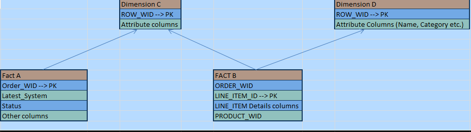
We have two facts and two dimensions which holds the below data:

Fact A : It consist of snapshot of Order’s latest footprint among several system. If we consider Order can go through several systems after being raised in ERP system (let’s say SIEBEL), then Fact Table A will store the latest status of Order in respect of which system it is in. So the primary key of this Fact is Order.

Fact B : It consist of the Line items of any Order and their individual status. Primary Key of this fact is Order Line Item.

Dimension C : It consist of an Order’s attributes e.g. Id, Geo information, Category etc.

Dimension D : It consist of Product’s attributes e.g. Name, Category, Model etc.

A typical data model for above scenario should look like below

If we now consider the business requirement – we need measure from Fact A and Fact B and attribute details from Dimension C and Dimension D. And probably you have already figured out the above depicted data model won’t be able to yield the intended result in OBIEE as we have one dimension table (D) which is non-conformed dimension i.e. Dimension D is not joined with Fact A thus it is not commonly accessible by both Facts A and B.

As we always say “All Road Lead to Rome” – one of the many approaches could be add product attributes (from dimension D) in Fact B as they are 1:1, there won’t be any inconsistency, but then we will have a liability to change Fact B table (PRODUCT related information) every time those product attributes get changed in Dimension D. This process can be handled by Auxiliary process as reckoned by ETL experts. We would love to discuss about this auxiliary change data capture process in future posts.

What if we decide to go with most logical data model depicted above and let us check we can handle it in BI (OBIEE in this case) and what are the consequences.

If we consider Fact A as our Driving Fact table then we can add the joins between Dimension C , Fact B and Dimension D e.g. C.ROW_WID = B.ORDER_WID AND B.PRODUCT_WID = D.ROW_WID into the same Logical Table Source under Logical Table of Dimension C

LTS for accommodating other tables

As we can see in the above diagram we have added the other tables in LTS, let us assume we had used Left Outer Join to neutralize few data nuances and one thing worth noticing is we have changed the Priority Group value other than default (value 0).

But this solution has a consequence as well. If we take any column from this logical table OBIEE will generate physical query with these 3 tables (Order , Order Item and Product). Now we can imagine that the physical sql will cause the performance overhead even for the simplest report. Ideally the simplest report should be able to generate its record-set from the below LTS configuration.

Simplest form of LTS

Please  note here the priority group is set to default value 0.

So we have the option of two set of LTS configuration as depicted in above examples. And we have seen that every option has its own merit and demerit as well , so which option we should choose?

To answer this question we should consider the option of method overriding we have seen in Object Oriented Programming world, I would discuss this approach in detail in my next post.

Hope you have enjoyed reading this post. Please share your comments and feedback.

Happy reading..Cheers!!

How to achieve almost 100% availability of BI reports even if when ETL is running – Synonym Toggling Technique – Part 2

We have discussed about concepts and a bit of theory behind synonym toggling in my previous post here.

In this post we would like to discuss about the technique of achieving this . Though there are several roads leads to Rome, I would show you one technique how I had approached the solution which worked absolutely fine for me

We will use one Oracle Dictionary Table – USER_SYNONYMS which hold synonym reference information.

Let us create two table with same structure as discussed in the previous post:

Here we have created two tables SYN_TOG_TEST_SYN1 and SYN_TOG_TEST_SYN2 with similar structure .

Then we have inserted one dummy record into each of those two tables so that we can differentiate while selecting from the synonym, looking into the data only.

Let us create one synonym on one table, we have created the synonym on _SYN1 table.

Test Table and Synonym Creation

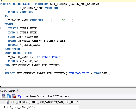
Then we have created one tiny utility for getting underlying table name for any given synonym. We would not discuss the generic function definition, as that is pretty self explanatory.

Get Current Table for Synonym

Then we have created one lookup table to maintain the references of synonym

Lookup Table

Then we have created synonym toggling main procedure

Toggling Procedure

Whoa!! we’ve now got everything we need to achieve ~ 100% availability of data into our enterprise reports. an working algorithm should somewhat look like the below:

Implementation of Synonym Toggling

Step 1: Get Current Table Name  for a given Synonym

Step 2: Get other table name for that synonym and current table from lookup table

Step 3: Truncate and insert into other table with complex aggregation / calculation. This step ensures that report is still pointing to old instance while ETL load data into new instance. This step is necessary for ETL load scenario, as we were testing with dummy tables, this step is not necessary.

Step 4: Command synonym to change its reference which we call Synonym Toggling here.

Step 5: Do not forget to test it whether you are getting latest data.

Now we have implemented Synonym Toggling in Oracle environment.

Hope you have enjoyed this post. Please  feel free to post any feedback or question in the comment section. Would love to hear your thoughts on this.

Thanks for reading..cheers!!

How to achieve almost 100% availability of BI reports even if when ETL is running – Synonym Toggling Technique – Part 1

We often see in BI Data warehouse projects, few mission critical reports across the whole reporting system. And those reports needs much more frequent data refresh as well.

In typical Data Warehouse reports we get the data from underlying Facts and Dimensions, in case of transactional OLTP driven reports we sometime configure BI to directly query the source tables to get more real time data – in all cases data should be available all the time in those reports, i.e. reports should not be blank (or no result found).

Lets say in one of those situation we came across with conjugation of necessity of a physical aggregate table on top of Fact table. Interesting point is – dimension and Fact tables can be populated with no downtime (i.e. we can Merge the data with existing Dimensional or Fact Data in those tables), but Aggregate tables rolls up the data in different attributes and often needed full refresh instead of incremental or delta refresh.

While doing the aggregate full refresh we first truncate the table then insert into that table with some aggregated query (using count(), sum(), min(), max() etc.). If your aggregated data calculation and insertion takes few minutes (lets say 10-15 minutes) we often end up in a situation where we can not show summary reports for those 10-15 minutes time period as our summary reports are coming from pre-calculated rolled up aggregate tables. There are many examples where you can read why we need aggregate navigation and how we can achieve aggregate navigation , I have found Mark Rittman’s blog very useful and explanatory.

Now that we are aware of the problem, lets discuss the resolution approach.

We can achieve the workable solution using Synonyms in Oracle. In simple word , Synonym works as a reference to a particular physical table and it can refer to only one physical table at a given instance

Relying on the above characteristics we can toggle between multiple physical tables.

Let us now focus how we can solve the above problem using synonym toggling.

Lets say our target aggregate is a synonym instead of a physical table. If we can create two same structured physical table then the aggregate synonym can be toggled between those two physical tables. If we can build any generic mechanism where we can change the synonym reference to one physical table alternatively in each ETL Load, then there would be hardly a second of downtime of those mission critical report from customer perspective.

I have tried to depict the concept in below diagram:

Synonym Toggling technique

Let’s assume we have a Synonym Target which is currently pointing to Physical Table 1 (which have the latest updated data) and our report points to Synonym Target, in next ETL run we should load the data in Physical Table 2 and at the very end we should toggle the Synonym Target’s pointer to point  Physical Table 2 where we would find the latest updated data.

Now if we use the Synonym Target as our aggregate table and with each ETL run if we change the pointer to alternative physical tables, then we can achieve  almost 100% availability of data in our reports.

I would post the technical bits (generic automated mechanism of synonym toggling) of the above depicted concept in my next blog.

Hope you have read the blog and found that useful. Please share your valuable thoughts and how you have overcome the situation in your real project scenario.

Also feel free to share any feedback or comments about this blog as I have just started blogging from today!!!

Have a good time. Cheers!!